Formation Outils Informatiques - Équipe NSE
Documentation Suite à la Formation
Présentations de la formation
Les slides, convertis en PDF: Slides
Cheat sheets
Liste de références
Un ensemble de liens utiles pour en apprendre plus:
Les slides, convertis en PDF: Slides
Un ensemble de liens utiles pour en apprendre plus:
The easiest way is to install qmusclesim via the anaconda distribution
The qMuscleSim package provides several tools which can be run all together from the main program or separately.
To run the simulation interface, simply type in a terminal:
The visualisation tools can be run using one of the following:
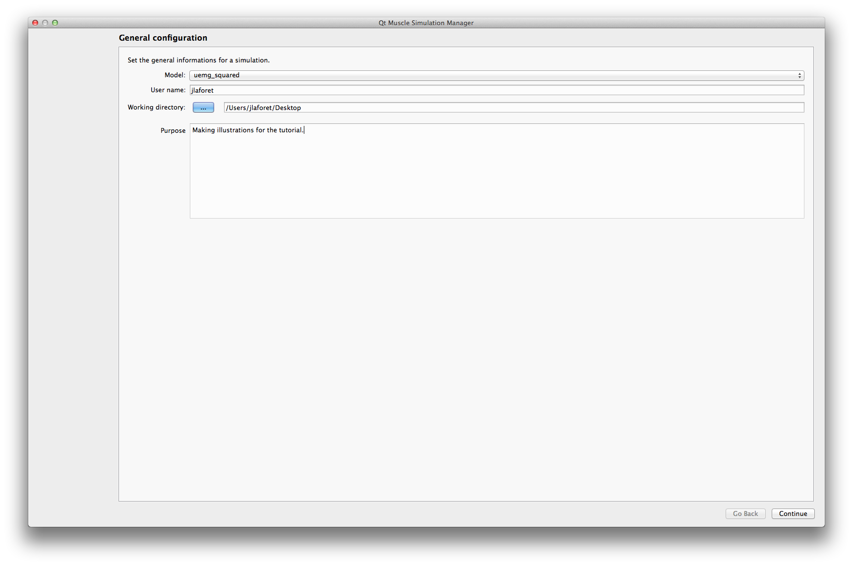
Model: Select the model you wish to simulate (among which have been detected on your system)
user name: Your name, as it will appear on the results report (defaults to your login on the current session)
Working directory: Directory where the simulation results will be saved. A subdirectory with a timestamp will be created here.
Purpose: A short description of the simulation and its purpose.
Here you can either load an existing json description or build your own.
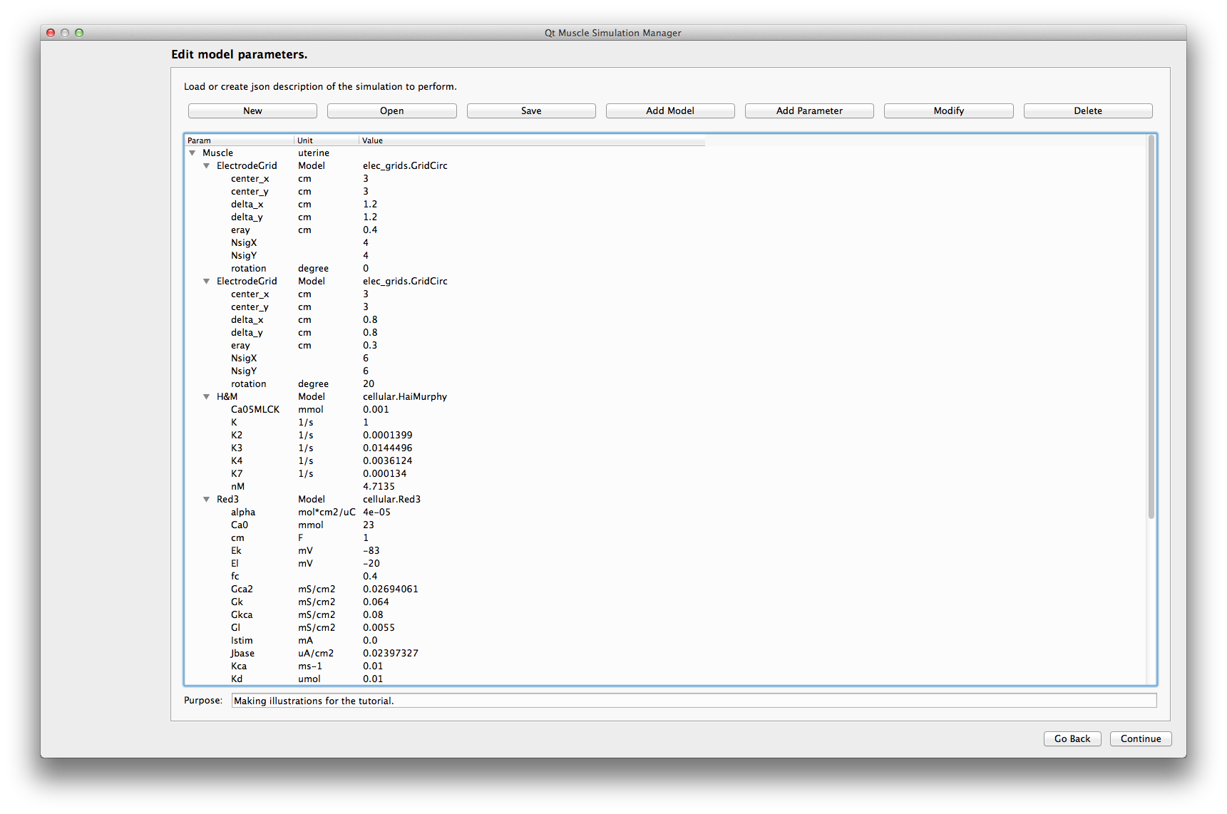
The buttons at the top of the interface give access to the main functions of this part:
New Creates a new empty description of the current model.
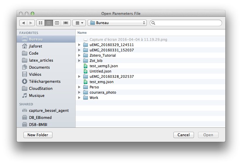
Open Opens an already existing json description. It can be altered afterwards.
Save Saves a copy of the description in json format. You must save your description before being able to run it.
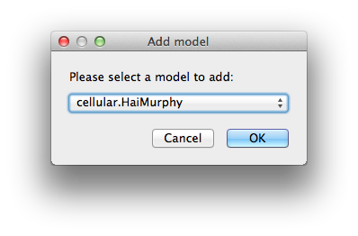
Add model Adds a new model with its default parameters. Please pay attention to the consistency of your description.
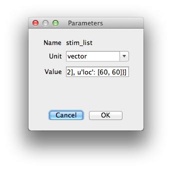
Add Parameter Adds a new parameter to the currently selected model. Please pay attention to the consistency of your description.
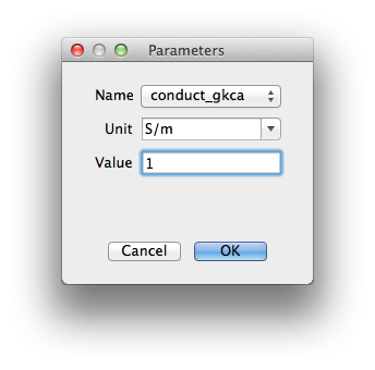
Modify Parameter Modify the currently selected parameter.
Delete Removes the currently selected paramter or model.
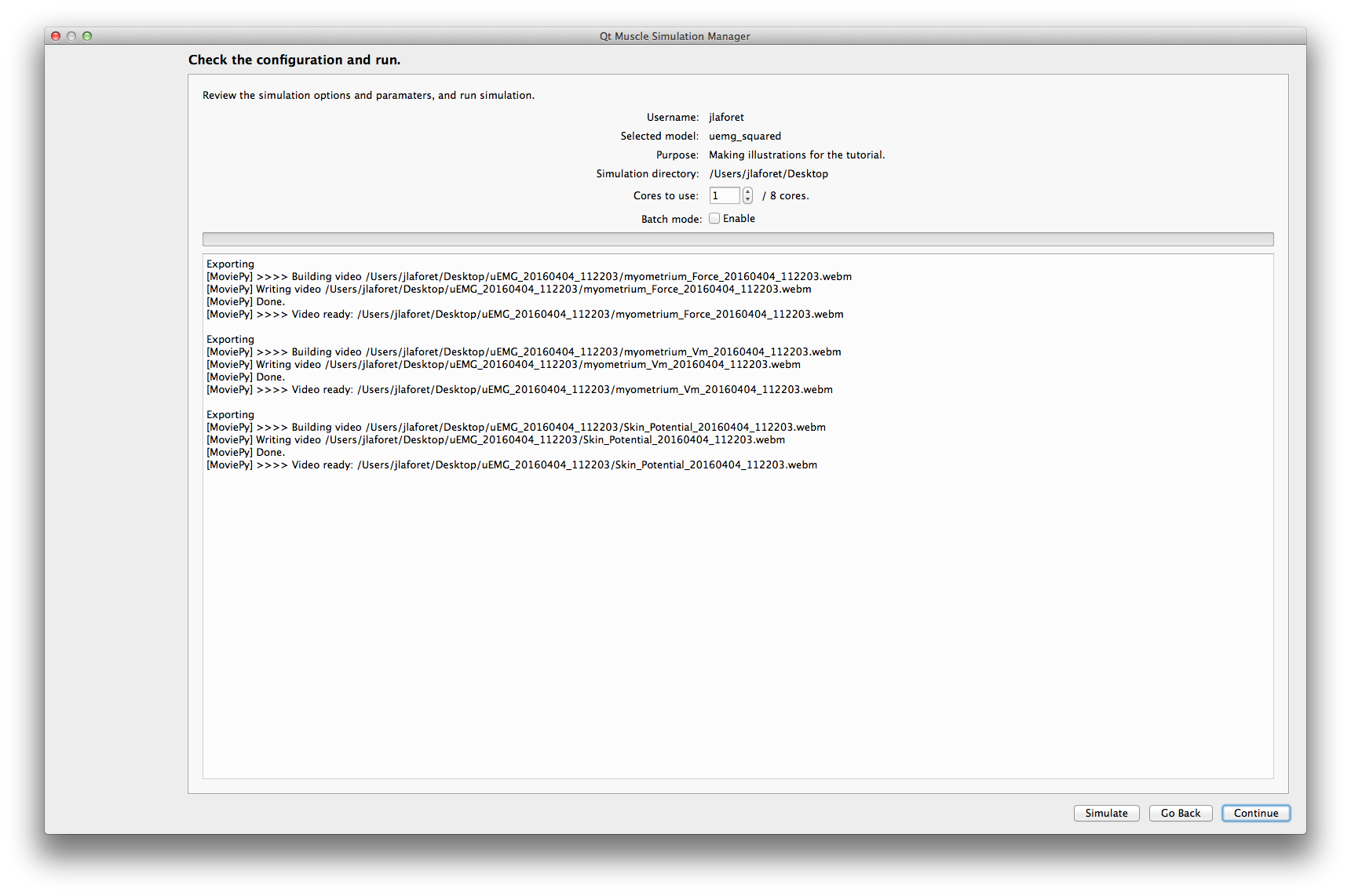
The interface displays the parameters entered at the first step and the simulation options:
Cores to use : Select the number of cores of your cpu to use for the simulation. This has no effect if the model doesn't support parallel computations.
batch mode If enabled, a simulation in batch mode will only save the EMG signals (if any) and will not produce graphical outputs.
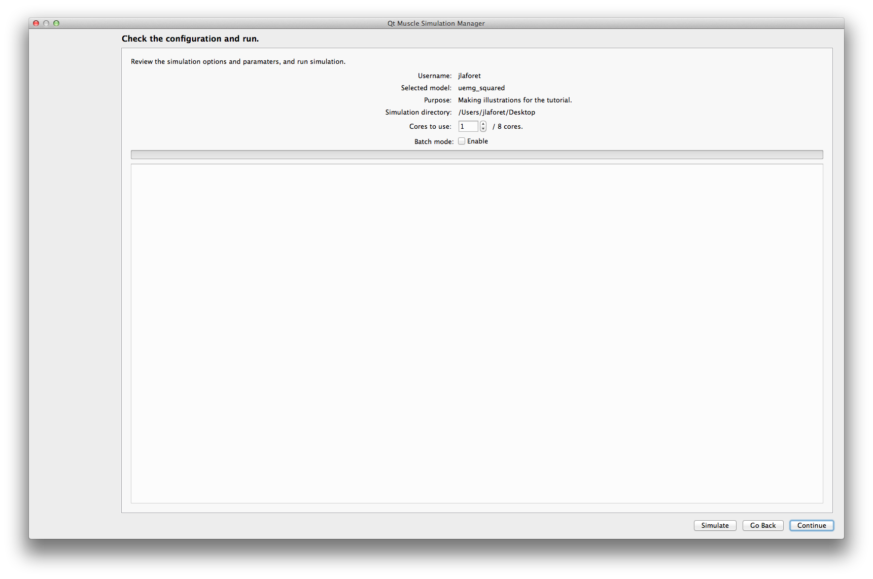
Simulate Runs the simulation. While the simulation is computing, the interface will display a busy progress bar.
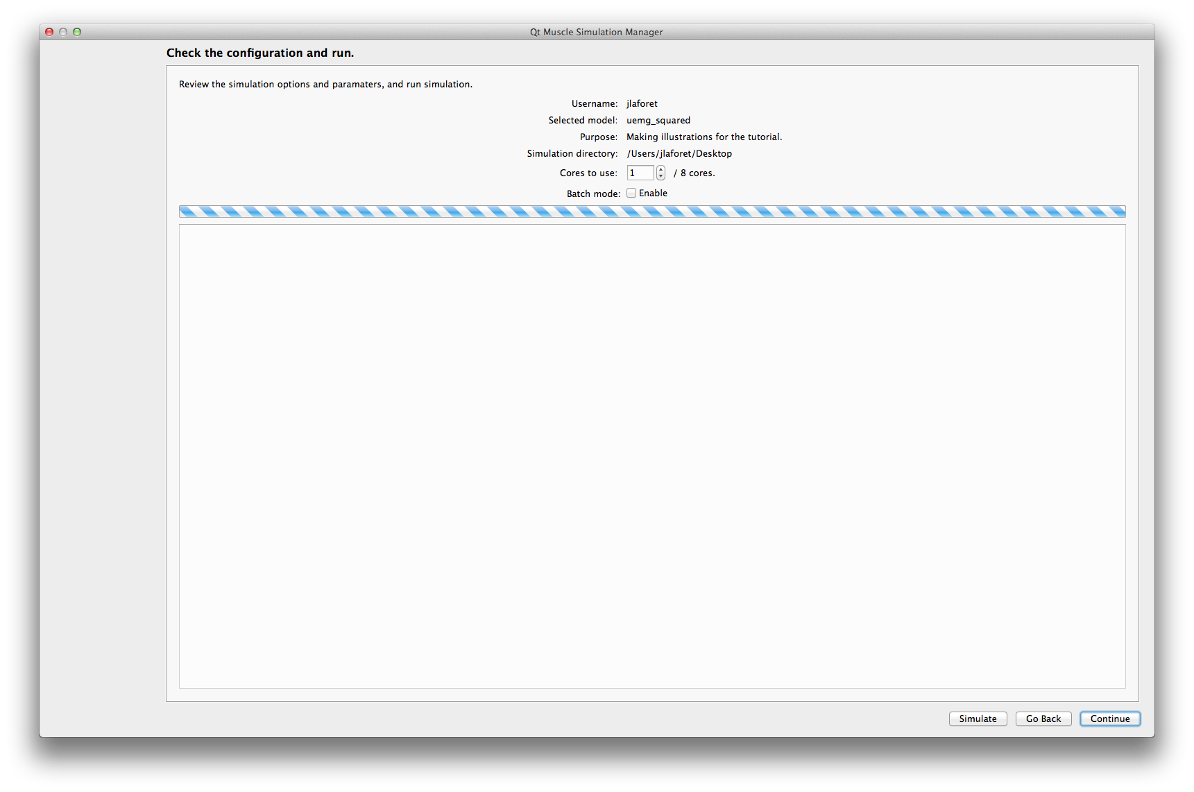
The complete progress bar is only displayed in the terminal. It also computes the ETA (Estimated Time of Arrival) of the simulation. .. image:: /tuto_qmusclesim/2_run_progress.png
The interface will also display any information or error messages generated by the model during the simulation.
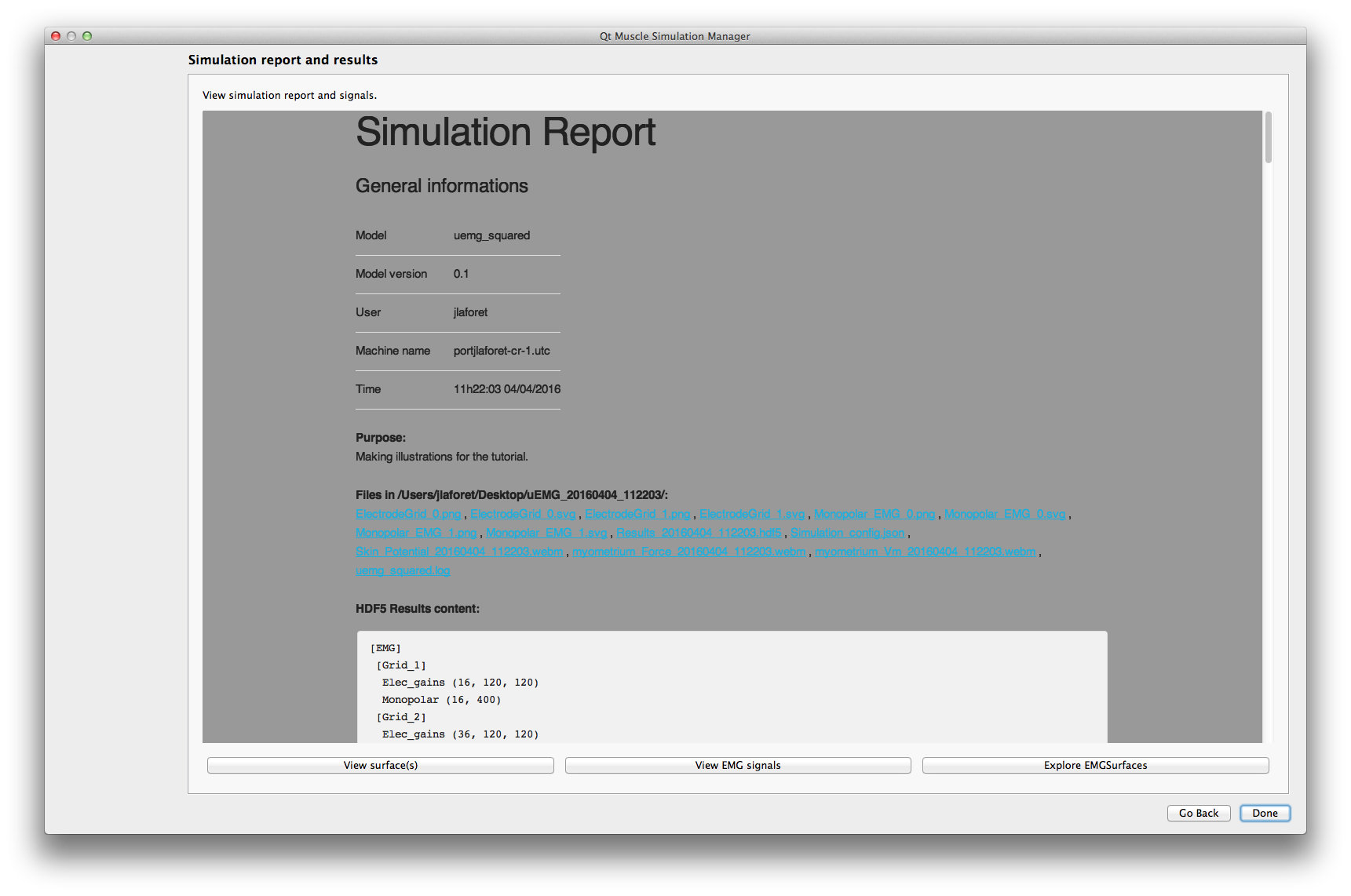
This last step display the html report of the simulation. The buttons at the bottom are links to the visualization applications provided by qMuscleSim. Only the applications pertinent for your data will be enabled. For example, if you only have EMG signals, the surface visualization will be disabled.
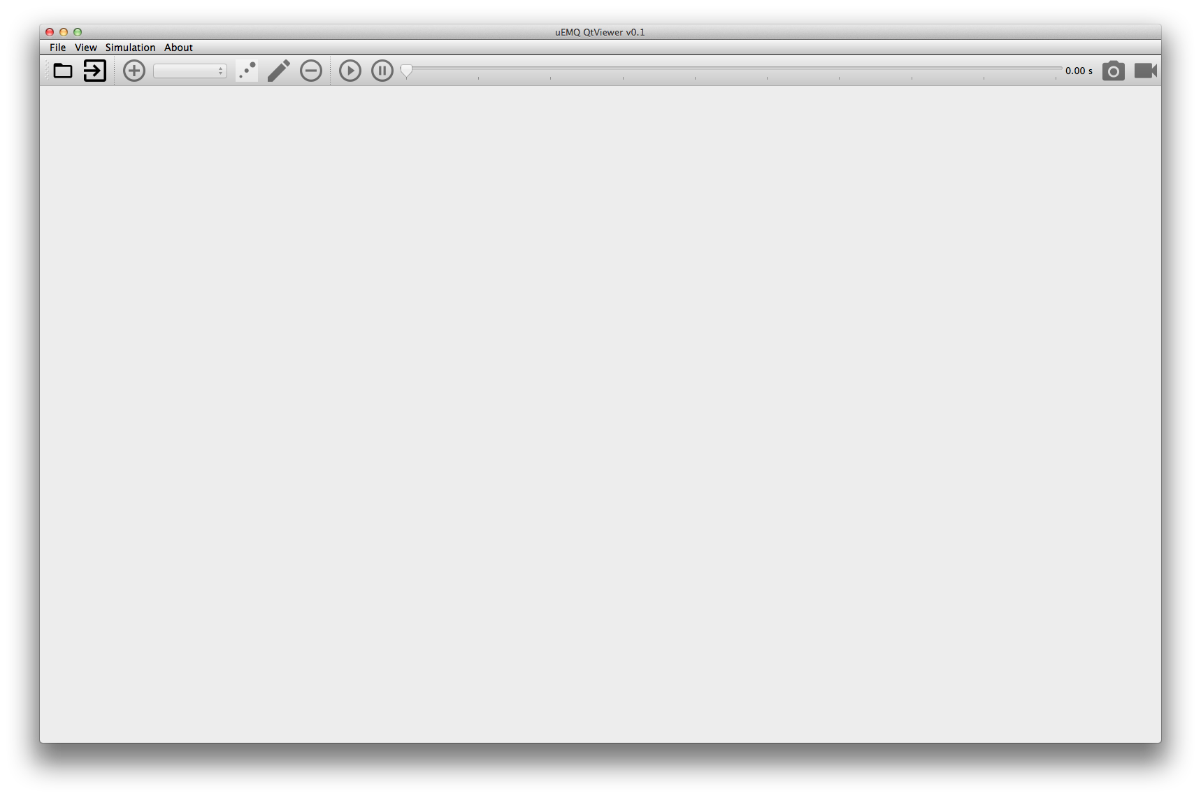
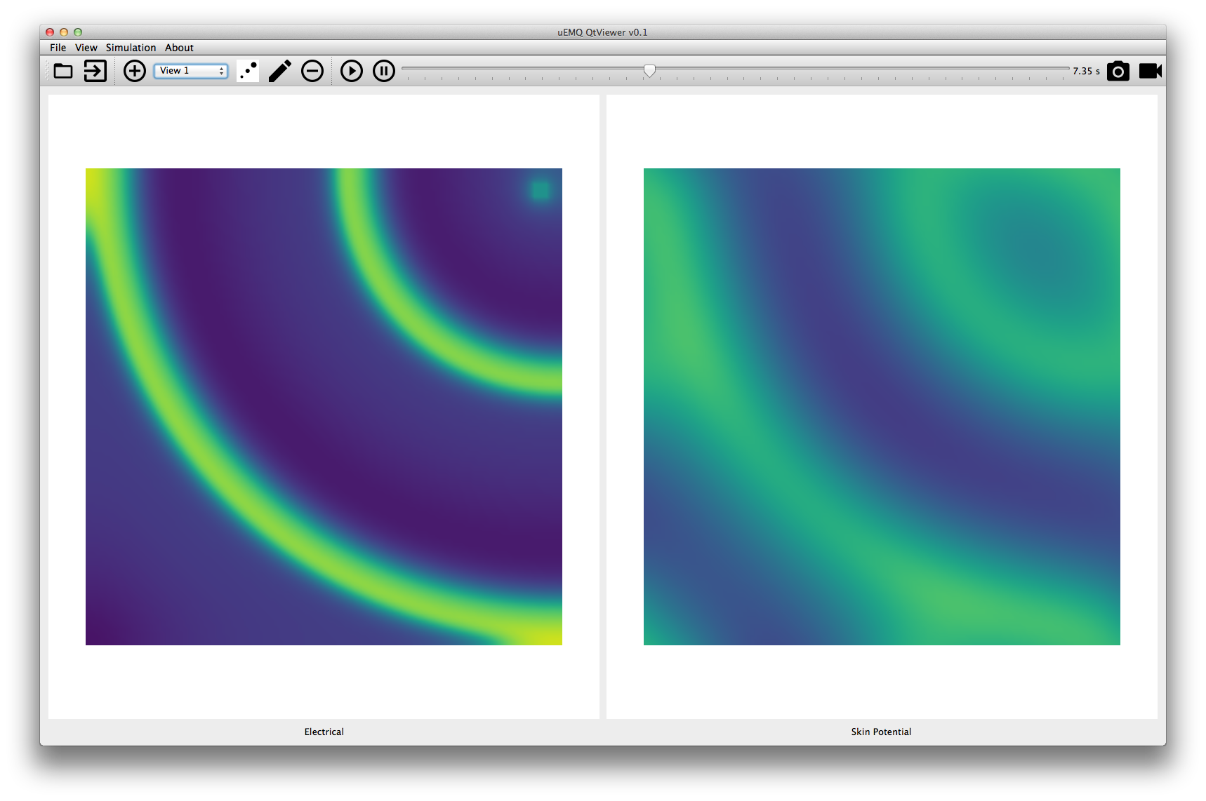
This application let you visualize surface data generated by your model simulation. To make comparisons, you can display several surfaces from the same simulation.
First you'll need to open the hdf5 results.
The add view dialog lets you define which surface and how it will be displayed.
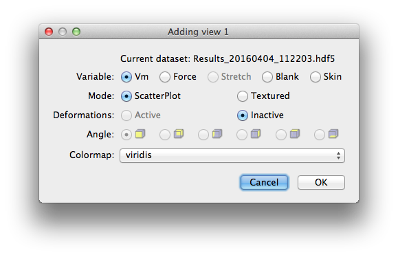
You can then visualize the evolution over time, and save pictures and videos.
This application will display the EMG signals simulated. First you'll need to open the hdf5 results.
The application allows you to visualize the signals for each grid simulated. You can also zoom and pan on the temporal scale (all channels will be affected).
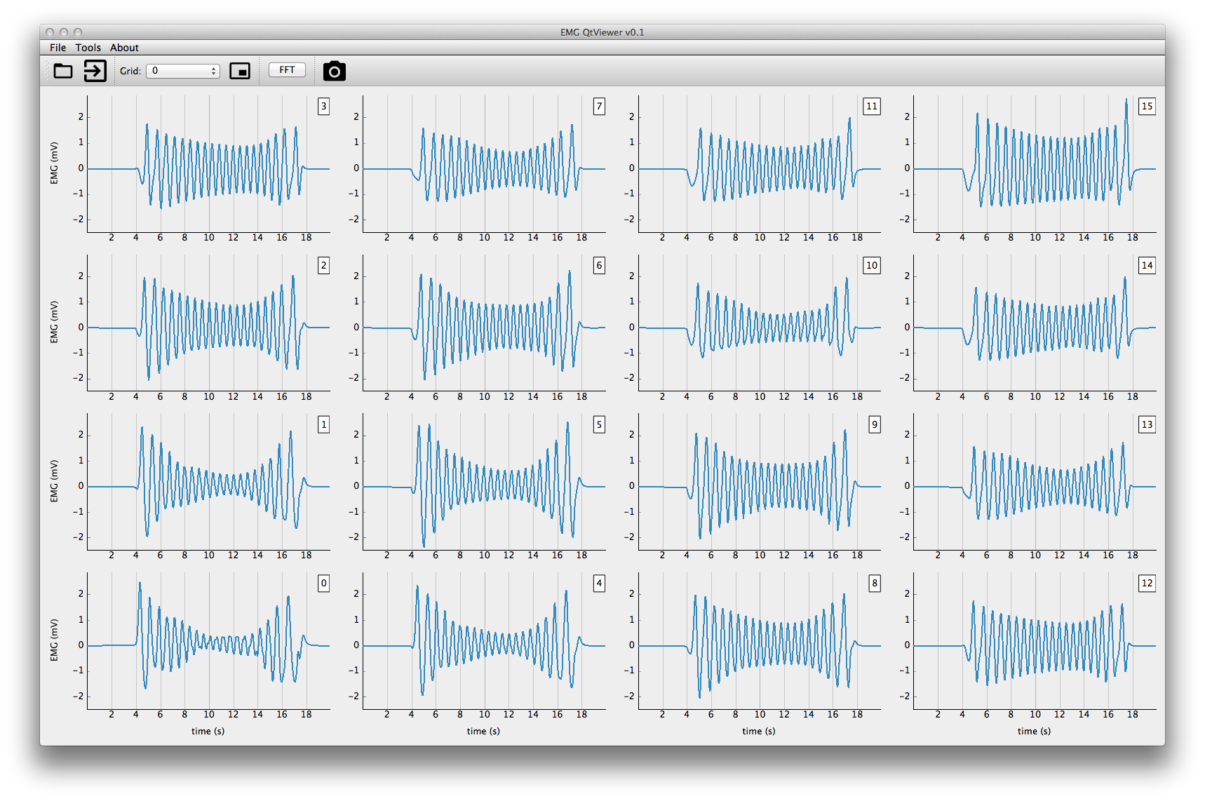
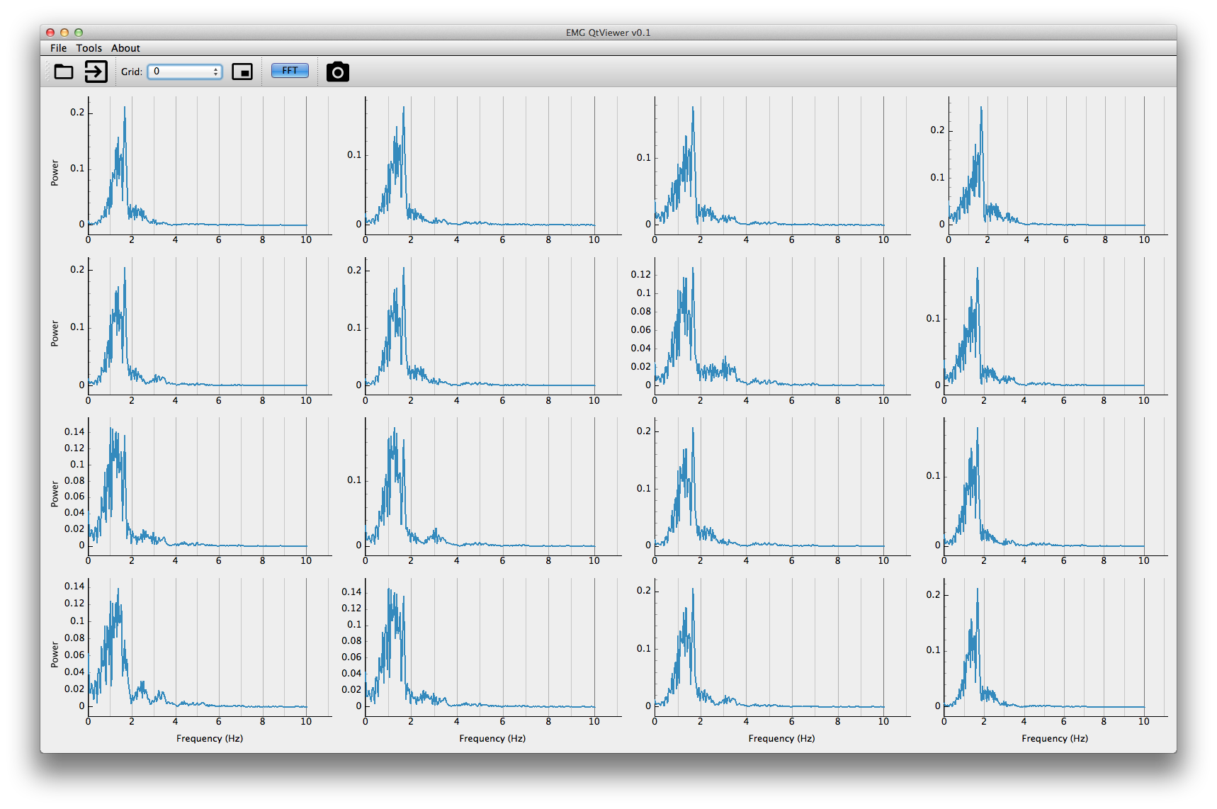
Pressing the fft button will toggle the power spectrum mode. Press it again to disable it.
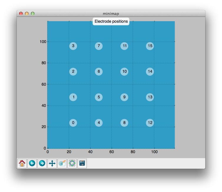
A map of the electrode grid is available by the minimap icon.
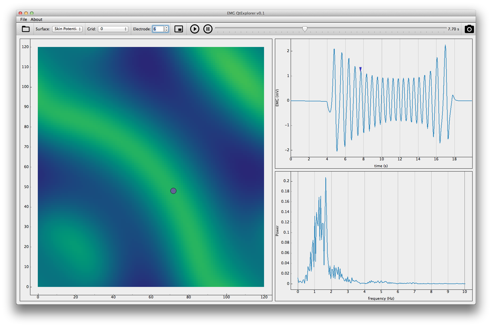
This last application offers a mixed visualization. It will display side by side a flat 2D surface and one channel of an electrode grid with its power spectrum. The controls are the same as previous applications.
Les deux séries de slides, convertis en PDF:
Un ensemble de liens utiles pour en apprendre plus:
PySens Tutorial / Basic Test==================
import json
import pysens
%pylab inline
First let's define our parameter space in json format. You should describe each parameter variations with a probability distributions.
As a test we will use the Ishigami function implemented as a basic test in the library.
%%writefile ishigami.json
{
 "model": "test",
 "parameters": [
   {
     "name": "X1",
     "distrib": {
       "max": 3.14,
       "min": -3.14,
       "type": "uniform"
     },
     "unit": "mm"
   },
   {
     "name": "X2",
     "distrib": {
       "min": -3.14,
       "max": 3.14,
       "type": "uniform"
     },
     "unit": "V"
   },
   {
     "name": "X3",
     "distrib": {
       "min": -3.14,
       "max": 3.14,
       "type": "uniform"
     },
     "unit": "V"
   }
 ]
}
Now we can sample this space using one of the available methods in pysens.sample
smpl=pysens.sample.Sobol('ishigami.json')
smpl.build()
Let's visualise our DOE and print its statistical properties:
smpl.plot_plan()
pysens.tools.print_stat(smpl.mat)

Now we can evaluate the model at each of the point described by the DOE plan:
ev=pysens.evaluate.TestIshigami('ishigami-Sobol.csv')
ev.simulate()
This generated a hundred npy files each containing the results of one evaluation of the model. They have been stored in a new subdirectory named by the time and date of the analysis.
(In the following lines, we use the name of the subdirectory stored in ev.subdir. You can run the post-processing and analysis without the evaluator object, just by giving the directory name instead.)
prcss=pysens.process.TestModels(ev.subdir)
Now we have both the DOE plan in ishigami-Sobol.csv and the features in Out.csv. Both files are in the subdirectory. For the test models, there's only one feature, the scalar output of the model.
Let's compute the linear correclations of the inputs / output:
anls=pysens.analyse.CorrelationsSA(ev.subdir+'ishigami-Sobol.csv',ev.subdir+'Out.csv')
anls.analyse()
anls.save_results()
anls.plot_results()


